Section 2 Differences between conventional calculation (ABC analysis) and Tera calculation |
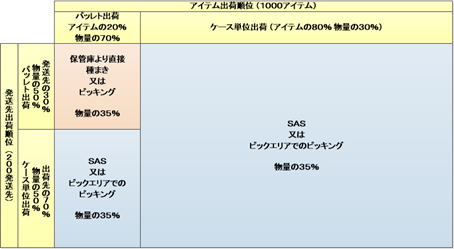
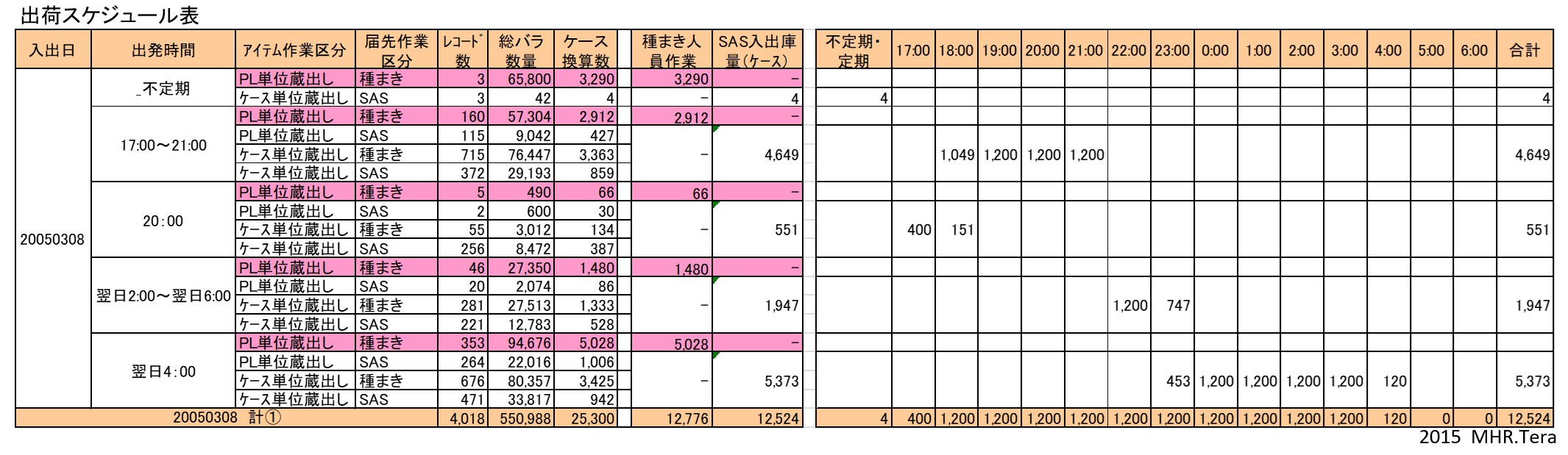
| In Tera calculations, calculations that use the ABC analysis method to tally data are called conventional calculations. ABC analysis divides ranks into thirds and performs tallying by rank and by shipping destination, while Tera calculations divide ranks into fifths and performs tallying by rank and by shipping destination. In conventional calculations, the totals for each item in the item tally and shipping destination tally are the same, but there is no correlation between the two tables. Therefore, conventional calculations cannot obtain information from these two tables about the shipping destination rank to which products with item rank A1 are allocated. When considering distribution center size and operation methods, or calculating logistics volume for each process, data that associates shipping destinations with items is required. Tera Calculation proposes a method of associating "time rank" with "shipping rank" and dividing and aggregating into 25 blocks (item rank 5 x shipping rank 5). In Tera Calculation, this aggregation table is called an EIQ matrix table. Tera Calculation is also designed to display the number of rows (number of issues), number of loose items, case conversion, PL conversion, volume conversion, and weight conversion, all separated by the same rank. By looking at this matrix table, for example, When an A1 rank item is stored on a flow shelf installed in the shipping work area, it is easy to calculate how many times it will be picked, what the total number of loose items is, what the volume is at that time, how many shipping containers are required, how many cases will be required to replenish the flow shelf from the storage area, and how many pallets will be required when it is transported from the storage area using a mixed PL. |
Section 3: Reflect shipping time, shipping route, shipping category, and item category in the calculation |
| Shipping data items include shipping time, shipping route, shipping category, and item category. Shipping time is divided into hourly intervals, and you can specify a time in the extraction condition settings of tera Calculation 1 to calculate within the specified range. This item is useful when determining whether forward loading is possible, and when investigating the volume of goods to be moved forward during certain time periods. It can also be used to create truck dispatch schedules based on the volume of goods by time period. Shipping route information includes information on where in the shipping space the shipment will be collected and which truck it will be loaded onto, such as the category for loading groups of goods going in the same direction on your own company's delivery, the courier category, or the carrier category. Shipping category information includes information on the relationship between your company and the destination, whether the goods will be shipped in a container or cardboard box, and classification information such as the company to which logistics processing will be requested, such as tagging. Item information includes the classification required at the time of arrival. For example, if the goods are outsourced, they may require quality inspection, or if they are received at your own factory, they may be received by your own delivery. |
![]() |
This EIQ matrix table clearly shows which group the shipping destination and product are in. It also allows you to calculate which items to replenish in the picking area (SAS) and when. |

Section 6. Examples of application of EIQ matrix spreadsheets |
| The EIQ matrix can be used to consider the shipping method for products or shipping destinations. The key to deciding on the shipping method is the volume of shipments. An EIQ matrix is a table that lists shipping destinations and products in order of the volume of logistics. In the above table, items and shipping destinations with a volume of 0.5 pallets or more/PIC are designated as pallet shipments. This pallet shipment group is inefficient for working in the picking area or SAS, but is efficient for sowing and can be processed in a sowing area for two or three shipping destinations. Groups other than pallet shipments are best stored temporarily in the picking area and picked from there, and are also groups where SAS can be useful. |
Section 2: Which shipping date should be focused on for aggregation? |
| Tera Calculations 1 and 2 can be calculated regardless of the shipping date selected. Increases or decreases in logistics volume on the shipping date will affect the results of the shipping data analysis and the distribution center size calculation. When it comes to logistics equipment, importance is placed on storage volume, inventory inbound and outbound, and the hourly processing capacity is typically considered based on peak times on shipping days with high volumes. However, selecting a shipping date with high volume when calculating distribution center size will result in a distribution center that is larger than necessary. Distribution center size should be calculated based on the overall shipping data average, rather than the selected shipping date. This is because on busy shipping days, shipping is made from safety stock. Safety stock is an inventory setting that provides security in the event of a delay in arrival or a decrease in incoming volume, but it is also used for fluctuations in shipping volume. Another reason is that when calculating using a specific shipping date, information about items that do not ship on that shipping date is not reflected in the calculation. Large-volume destinations often have fixed shipping days, and items are shipped at regular intervals. Therefore, high-flow items may become low-flow items or may be omitted from shipping items. By including all data, information on all items can be obtained. Tera Calculation 2 sets the Tera setting to the overall average of the shipping data. Tera Calculation takes about 5 minutes to run, so one method is to calculate the distribution center size for each shipping date and then take into account changes in shipping volume and size, as well as future volume, to determine the size of the distribution center. |
Section 1 EIQ Matrix Summary Table |
| In the EIQ matrix table, the display unit "loose" means the number of loose items, "case" means case conversion, "PL" means PL conversion, "volume" means volume conversion, and "weight" means weight conversion. From now on, please note that all quantity units other than "loose" are conversion units converted from the number of loose items (when the term "case" appears, it means case conversion). As mentioned above, the EIQ matrix table is a summary table divided into 5 * 5 = 25 blocks, and the horizontal total is the summary of destination shipment volume, and the vertical total is the summary of item volume. If the EIQ matrix table uses PL conversion for display units, the horizontal total will match the PL conversion of the conventionally calculated item summary, and the vertical total will match the PL conversion of the conventionally calculated shipping destination summary. The matrix summary and conventional calculation are linked and always display the same content. The same is true for the number of shipping destinations and items. Ideally, a system should be designed by looking at the volume of which items are being shipped to which destinations, and Professor Suzuki Shin introduced this as the EIQ table. It's certainly possible to create and analyze an EIQ table with around 50 shipping destinations and 100 items. However, with an EIQ table like the shipping data in this example, with over 400 destinations and over 4,000 items, the table would be too large to fit on an 8-tatami room and would be impossible to read. At Tera Calc, we've devised a way to aggregate EIQ tables by grouping them by rank, which we call an EIQ matrix table. There's also a way to display an EIQ table as a scatter plot by displaying points. 400 shipping destinations and 4,000 items are plotted, and by scrolling horizontally on a PC screen, you can visually see the distribution of the EIQ table. At Tera Calc, we call this a EIQ scatter plot. Next, we'll introduce the EIQ graph devised by Professor Shin Suzuki. This graph shows the cumulative volume of goods at shipping destinations and items as curves, and the number of shipments to shipping destinations and the number of shipments by item as bars, representing daily volume in a single diagram. Please refer to other copyrighted material for the EIQ table and EIQ graph. |