Section 1: Differences between conventional calculations and EIQ matrix calculations |
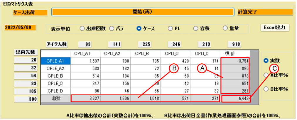
| In Tera calculations, calculations that use the ABC analysis method are called traditional calculations. ABC analysis divides ranks into three parts and performs item-by-item and shipping destination aggregations, while Tera calculations divide ranks into five parts and performs item-by-item and shipping destination aggregations. In traditional calculations, the totals for each item in the item aggregation and shipping destination aggregation are the same, but there is no correlation between the item aggregation and shipping destination aggregation. Therefore, traditional calculations do not know to which shipping destination rank a product with item rank A1 is allocated from these two tables. Data linking shipping destinations and items is required when considering distribution center size and operation methods and calculating logistics volume for each process. Tera Calc proposes a method of associating "time rank" with "shipping rank" and dividing and aggregating into 25 blocks (item rank 5 * shipping rank 5) . In Tera Calc, this aggregation table is called an EIQ matrix table. Tera Calc can also display the number of rows (number of issues), number of loose items, case conversion, PL conversion, volume conversion, and weight conversion, using the same rank divisions. Using this EIQ matrix table, for example, it is possible to easily read from the EIQ matrix table how many times an A1 rank item on the flow shelf in the shipping work area has been picked, what the total number of loose items is, what the volume was at that time, how many shipping containers are required, how many cases will be needed to replenish the flow shelf from the storage area, and how many pallets will be required when it is brought from the storage area on a mixed PL . In the EIQ matrix table, the display unit "loose |
  |
Difference between EIQ table and EIQ matrix table
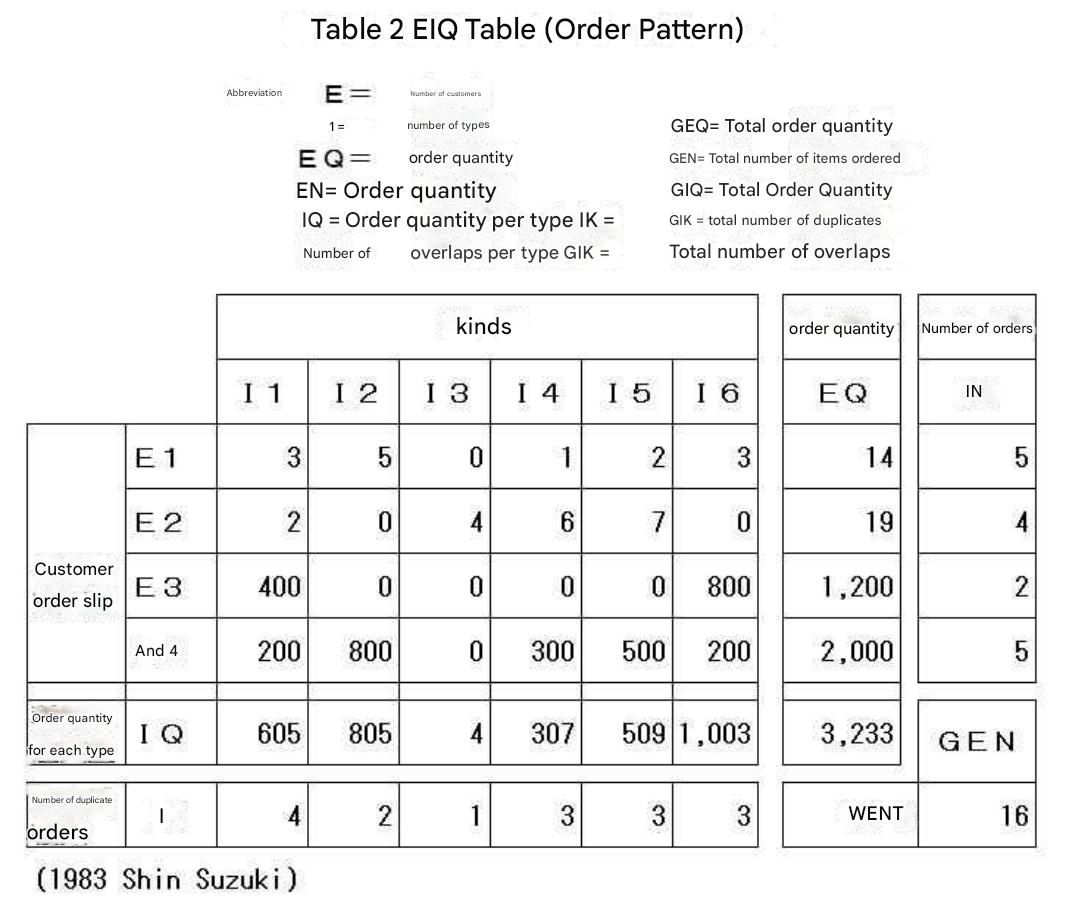
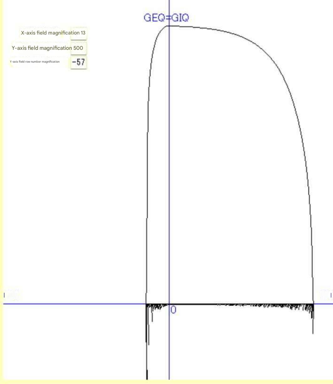
Ideally, a system should be designed by looking at the volume of goods that each item is sending to each destination, and Professor Suzuki Shin introduced this as an EIQ table. Another method is to display the EIQ table as a scatter plot. By plotting 400 destinations and 4000 items, you can visually see the distribution of the EIQ table by scrolling horizontally on your computer screen. In Tera Calc, we call this diagram the EIQ scatter plot (see Tera Calc 4_Reference EIQ). Next , we introduce the EIQ graph devised by Professor Suzuki Shin . This graph displays the daily volume
of goods in a single diagram, with the cumulative volume of goods at the
destination and the cumulative volume of goods per item as curves and the
number of shipments to the destination and the number of shipments per
item as bars. (See Tera Calc 4_Reference EIQ.) Please refer to other copyrighted works for the EIQ table and EIQ graph. |
Section 2: Relationship between conventional calculation and EIQ matrix calculation
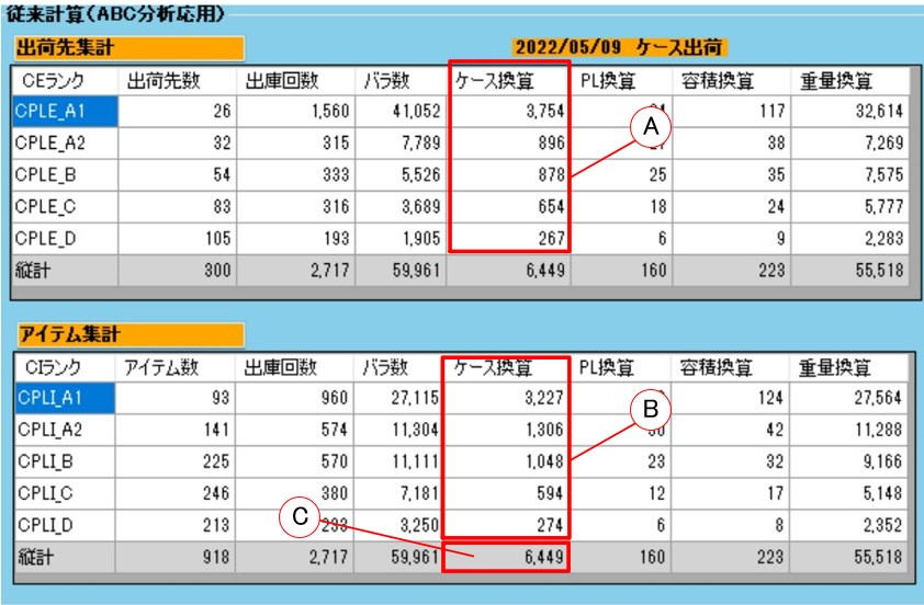 |
In conventional calculations, the shipping destination total and item total are calculated separately, so the relationship between the shipping destination total and item total is not clear. With the EIQ matrix calculation, the quantity of items A1 rank at the shipping destination A1 rank is known, and the quantity is calculated with the relationship between the shipping destination and the item. Observation : This EIQ matrix table makes it possible to grasp how much material flows from each item rank (equipment) to the shipping destination rank (shipping area). |
The EIQ matrix table allows you to specify extraction conditions and display data that meets the extraction conditions. It is often confusing to look at summary tables such as the A1 rank
of case shipment items , the A1 rank of case shipment destinations , the A1 rank of bulk shipment items , and the A1 rank of bulk shipment destinations . To eliminate this confusion, the table has been designed so that the contents of the table can be identified by looking at the rank symbol. The rank symbol " CKE_A1 " means the first letter, " C " for case shipment and " B " for bulk shipment , the second letter, the data item used for ranking, "row" for number of rows (number of shipments), "ba" for number of bulk shipments, "ke" for case conversion, "PL " for pallet conversion, "yoko" for volume conversion, and "ju" for weight conversion.
, and the fourth character, " A1 " is the A1 rank, " A2 " is the A2 rank, " B " is the B rank, " C " is the C rank, and " D " is the D rank
. Therefore, the rank symbol "CKEEA1" represents case shipment, rank calculation based on case conversion, and A1 rank for the destination rank.
When cutting out the observation
EIQ matrix table and pasting it into another document, be
careful not to write the "shipping method (case shipment)," "shipping date (2022/05/09)," and "display unit (case)" at the top of the cut-out table, as this will make it difficult to understand what the calculation is for
.
Section 5 Data Analysis and Aggregation
|
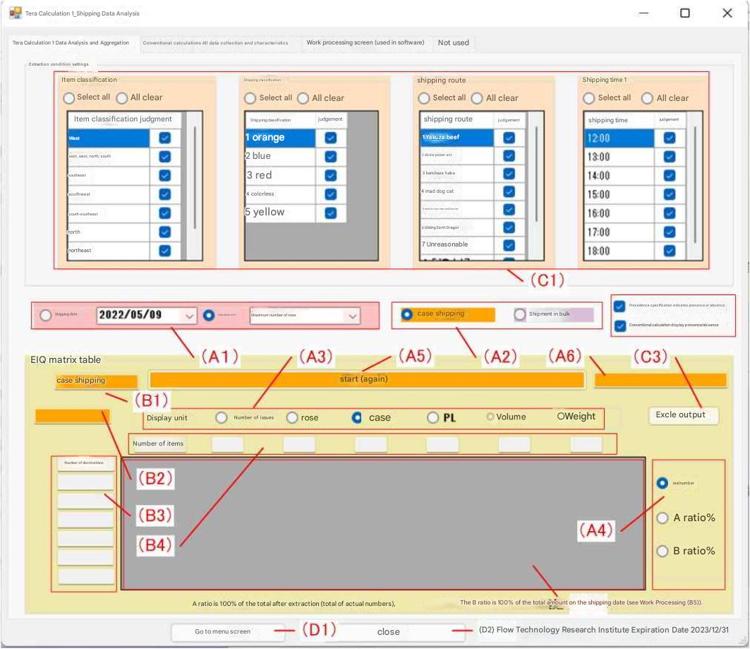 |
Click the radio button for shipping date in (A1) to specify the shipping date and perform aggregation. Click the radio button for characteristics to select the maximum row count date, maximum case shipping date, and maximum bulk shipping date. (A2) Use the radio button to select either case shipping or bulk shipping. (A3) Select one of six options for display unit (number of shipments, bulk, etc.) from the radio button. (A4) Select one of two options (actual number, % ratio) from the radio button. After selecting (A1) and (A4), click the start button (A5) to begin processing. The processing status is displayed in the text box (A6). After calculation processing, the case shipping or bulk shipping classification to be output is displayed in (B1), the shipping date, (B2), (B3) number of shipping destinations, and (B4) number of items are displayed, and the EIQ matrix table is output to the data grid view (table) (B5). |
| The matrix table can display actual numbers and ratio %. A ratio % displays the ratio of each rank with the total after extraction (total actual numbers) as 100%, and B ratio % displays the total of the total amount on the shipping date as 100%. (C1) Select targets from the four shipping condition items of the shipping data using checkboxes (multiple selections possible). Data for items with no checkboxes checked (shipping data records) are excluded and the EIQ matrix table is calculated. (C3) EXCLE output outputs the EIQ matrix table to EXCEL. |
|||||||||||
|
|